Did AI users beat AI sellers — and if so, why? A test of two explanations

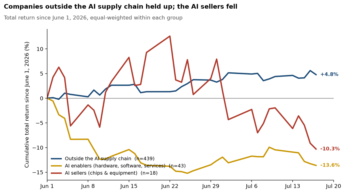
At the start of summer 2026, the companies that use AI outperformed the companies that sell it. Here is a clean way to ask why — and to find out.

• The “AI users beat AI sellers” story looks much less dramatic once you compare similar companies.
  At first glance, companies outside the AI supply chain beat chipmakers and other AI suppliers by about 15 percentage points. But most of that gap disappears after accounting for differences such as industry, company size, past stock performance, and risk. Much of what looked like an “AI users” advantage was really a group of high-flying technology stocks pulling back while the rest of the market held up better.
• There may still be a gap, but the evidence is not strong enough to call it a dependable investing trend.
  After those differences are taken into account, the gap falls to about 4 percentage points when users are compared only with chipmakers, and about 6 percentage points when they are compared with the broader AI supply chain. The second number is still meaningful, but it is not statistically convincing under the more appropriate test required for such a small group of suppliers. The result also changes depending on which companies are counted as AI suppliers.
• The data do not show that AI users won because AI was already improving their profits.
  Among companies outside the AI supply chain, those that had recently beaten earnings forecasts did not perform better afterward than those that missed. But this does not prove that AI is failing to improve profits. The earnings measure is limited: it was already public, it only records whether a company beat or missed, and it does not tell us whether AI caused the result. The finding only shows that, among these companies, a recent earnings beat did not predict stronger stock performance.

At the start of summer 2026, two groups of companies moved in opposite directions. The companies that sell the picks and shovels of AI — chipmakers and hardware firms — fell. Companies outside that supply chain held up or rose. In shorthand, “AI users” beat “AI sellers.”

That is not in dispute. The interesting question is why, because two very different stories fit the data, and they lead to very different conclusions.

Explanation 1 — AI is starting to pay off. The companies using AI are getting real benefits that show up in their profits, and investors bid them up for it. One observable—but imperfect—implication is that firms with recent earnings beats might continue to outperform.

Explanation 2 — the sellers just fell back to earth. The chip and hardware stocks had run up enormously beforehand and simply gave back some gains — an ordinary pullback after a big run. Under this story, the “users winning” pattern is largely a matter of composition: the users didn’t do anything special; the suppliers dropped.

The research question, in one sentence: did the non-supply-side firms out-return the AI suppliers because AI is producing better profits — or simply because the suppliers, which had run up the most, fell back the hardest?

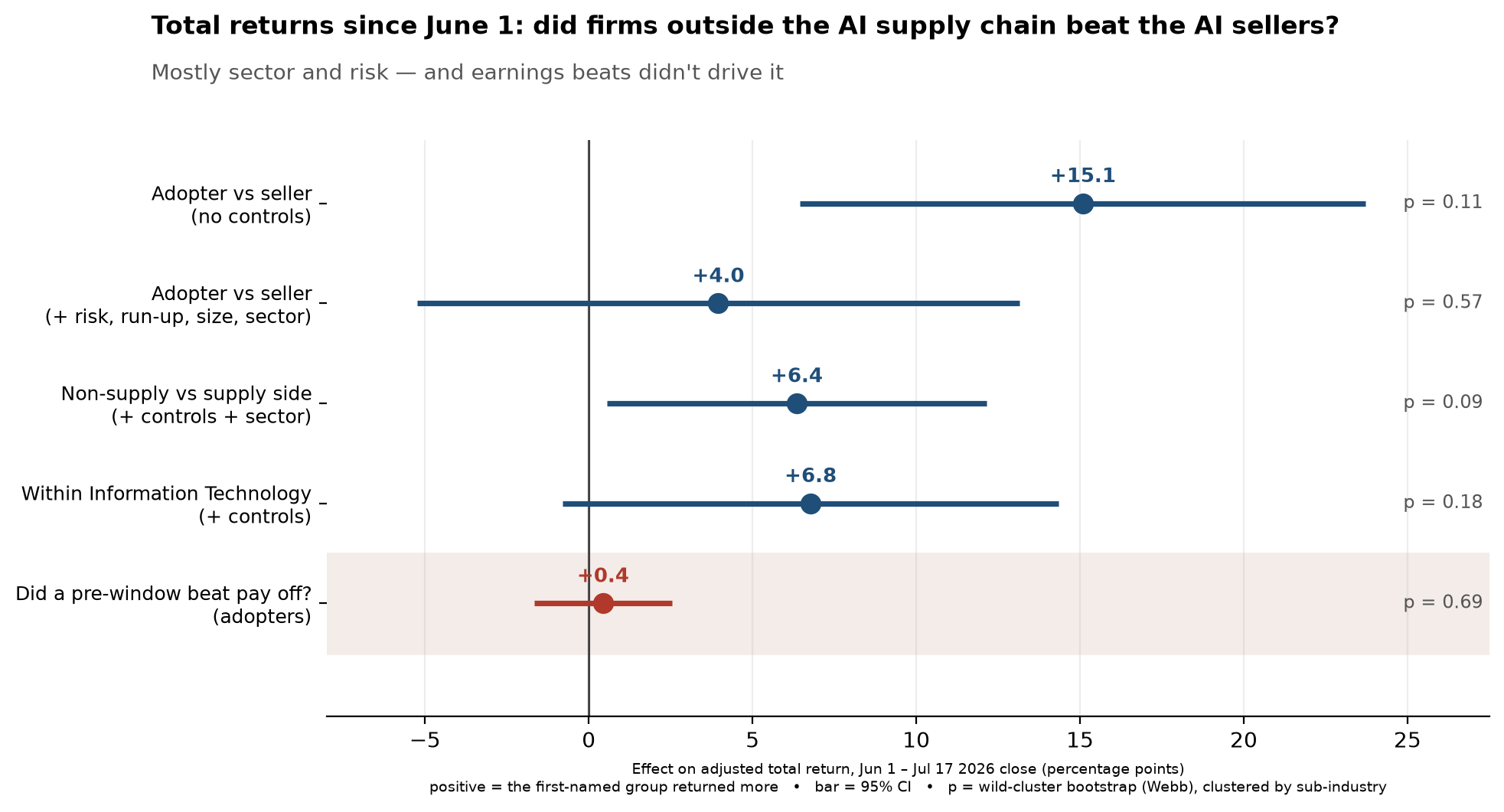
The verdict, up front. The observed gap is large. But most of it is absorbed by the combined effects of ordinary risk exposure, firms’ own price histories, size, and sector composition — the sellers are technology stocks, and the “users” are most of the rest of the market. After those controls, two comparisons remain. Against the 17 sellers alone, the fully-adjusted gap is +4.0 points and not statistically significant (bootstrap p = 0.57). Against the whole AI supply side with sector held fixed, it is +6.4 points — economically meaningful, but only marginal under valid few-cluster inference (bootstrap p ≈ 0.09). And the supplementary earnings test offers no support for Explanation 1: among the non-supply-side firms, a prior profit beat did not predict higher returns. This one window cannot support a strong claim in either direction — which is itself the useful result.

Hypotheses and how we test them

The two explanations make opposite, checkable predictions.

H1 (AI is paying off): the gap survives after we account for ordinary risk, recent run-ups, size and sector, and firms that beat their earnings forecasts out-return firms that miss.

H2 (valuation reset / composition): the gap is mostly explained by risk exposure, momentum reversal and sector, and beating forecasts is unrelated to returns.

Two tests separate them. First, does the gap between non-supply-side firms and AI suppliers hold up once we control for risk exposures, each firm’s own recent price run-up, its size, and its sector? If most of the gap is those factors, that favors H2. Second, among the non-supply-side firms, does beating earnings forecasts predict a higher return? This provides a limited supplementary test of H1, although the beat was already public and is not AI-specific; if it is absent, that specific channel finds no support in the data.

One honesty note on the second test. The earnings measure we can build from free data is a firm’s most recent profit “beat” reported before the window. That information was already public, is not specific to AI, and is recorded only as a yes/no. So a null result is informative but limited: it says a prior beat did not predict returns — not that AI-driven earnings were absent.

Data and sources

The universe is the S&P 500. We take the current constituent list and keep firms whose index-entry date is on or before June 1, 2026, so membership is set by the index rather than hand-picked. (This is a practical approximation, not a true historical snapshot: it cannot restore firms that were members on June 1 but were removed before the list was downloaded.)

Each firm is sorted by its GICS classification (the Global Industry Classification Standard, the MSCI/S&P system for grouping companies by industry) into a role in the AI value chain: sellers (semiconductors and chip-making equipment), enablers (the surrounding infrastructure — hardware, networking, enterprise software, IT services), and adopters (everyone else). “Adopter” here means simply a non-supply-side firm; it does not certify that a company uses AI heavily or effectively. Two documented overrides correct misleading labels — Apple, for instance, sits under “Technology Hardware” by GICS and is reclassified as an adopter rather than an enabler.

Stock prices, shares outstanding, and earnings surprises come from Yahoo Finance; the risk factors (the Fama–French five factors plus momentum) come from the Ken French Data Library. All sources are free and public, and the replication code is available.

Methodology

The outcome is each stock’s adjusted total return from June 1 to the July 17, 2026 close (the last trading day before the July 18 write-up). All return-based predictors are measured as of the beginning of the window. Company size uses the June 1 adjusted price multiplied by Yahoo’s currently reported shares outstanding; the price component is point-in-time, while the share count is an approximation because a clean historical count was unavailable from the free source.

We control for the things that could produce a gap without any AI content. Using the year of returns before the window, we estimate each firm’s exposure to the standard risk factors (market, size, value, profitability, investment and momentum) and its idiosyncratic volatility. We add each firm’s own trailing 1-, 3-, 6- and 12-month returns and its 12-month drawdown — a direct measure of how far it had run up — plus its size and its sector. Because a firm’s role is assigned at the level of its GICS sub-industry, and only a handful of sub-industries make up the supply side, we cluster the statistical errors by sub-industry and confirm the key result with a wild-cluster bootstrap, which is reliable when few groups carry the classification.

We test the earnings channel directly: within the adopters, we relate the window return to whether each firm beat its most recent profit forecast before the window, holding the full set of controls and sector fixed effects.

Intuition

The logic is simple. If AI is genuinely lifting profits at the companies that use it, that benefit has to travel through earnings to reach the stock price — one imperfect observable implication is that firms with recent earnings beats might subsequently outperform. That is a specific, testable prediction. If instead the whole pattern is the supply side unwinding a huge prior run, then earnings shouldn’t matter, and the “gap” is mostly the arithmetic of high-flying stocks reverting while the rest of the market sat still — with technology stocks concentrated on the side that fell.

Results

The raw pattern is stark (Table A1): adopters returned +4.8% on average over the window, while enablers fell −13.6% and sellers −10.3%. Note an early tension with Explanation 1: high pre-window beat rates did not insulate the supply-side firms from losses — sellers beat their forecasts 100% of the time and enablers 95%, yet both fell hardest.

Table A1. Adjusted total return and pre-window earnings-beat rate by role. S&P 500 firms with index entry on or before June 1, 2026; 498 with complete data. Window: June 1 to the July 17, 2026 close.

Does the gap survive controls (Table A2)? The raw adopter-versus-seller gap is +15.1 points. Adding the risk-factor exposures cuts it to +9.2; adding each firm’s own run-up, its size and its sector cuts it to +4.0 points, and it is no longer statistically distinguishable from zero (bootstrap p = 0.57). In other words, the risk, price-history, size and sector controls together account for roughly three-quarters of the raw spread.

The narrow adopter-versus-seller comparison rests on just 17 sellers, so we also compare adopters with the whole supply side (sellers and enablers pooled), with sector held fixed. That sector-adjusted gap is +6.4 points. Under conventional sub-industry-clustered inference it is statistically significant (p = 0.032), but that test may be unreliable because only nine sub-industries carry the supply-side classification. The preferred wild-cluster-bootstrap p-value is approximately 0.09, so the gap is best described as economically meaningful but only statistically marginal. It is also fragile: moving the software firms from the supply side to the user side cuts it to +3.7 points (p = 0.36), and the same comparison run within Information Technology alone is +6.8 points but not significant under the bootstrap (p = 0.18).

The supplementary earnings test also provides no support for Explanation 1. Among the adopters, a pre-window earnings beat was associated with a +0.4-point return difference, with a 95% confidence interval from −1.7 to +2.5 points and a p-value of 0.69. Firms that beat their forecasts did not out-return firms that missed. Because that beat was already public and is not AI-specific, this does not prove AI-driven earnings were absent — it is a possible earnings-related channel consistent with the “AI is paying off” explanation that simply leaves no mark here.

Table A2. What is driving the gap. Effect on the window return (percentage points), with 95% confidence intervals; errors clustered by GICS sub-industry. The p column reports wild-cluster-bootstrap p-values (Webb weights) — the preferred inference given few supply-side sub-industries; conventional clustered p-values appear in the note. Controls are defined in the appendix.

Notes: the p column is the wild-cluster bootstrap (Webb weights, clustered by sub-industry), the preferred inference because only nine sub-industries carry the supply-side classification. The corresponding conventional clustered p-values are 0.001, 0.080, 0.032, 0.079 and 0.685 for the five estimated rows; they are smaller because they understate uncertainty with so few clusters. The 95% CI is the conventional clustered interval (a different procedure than the bootstrap), so it can exclude zero even where the bootstrap p exceeds 0.05 — as in the pooled row. The “+ risk-factor exposures” row is an intermediate specification and was not bootstrapped (—).

Robustness: the sector-adjusted pooled gap holds its sign under a winsorized outcome (+5.9, p = 0.04) and leaving out any one sub-industry (range +4.1 to +7.9), but falls to +3.7 (p = 0.36) when software is reclassified to the user side, and is only marginal under the validated few-cluster bootstrap (p ≈ 0.09). The earnings-beat effect is a tight interval around zero.

Robustness: the earnings channel in event time

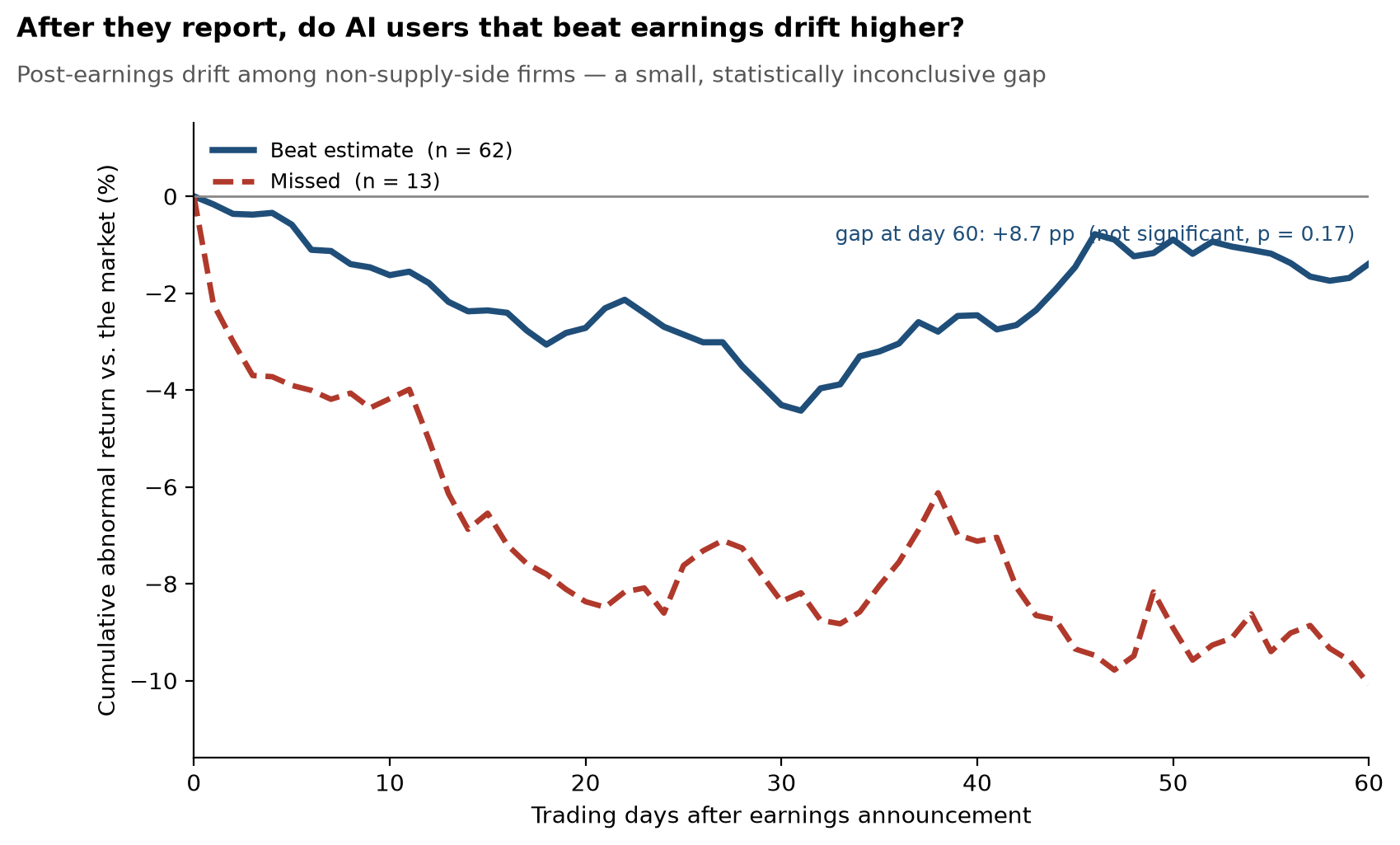
A reviewer noted that our earnings test uses a binary beat and a fixed calendar window, while post-earnings drift (Bernard and Thomas, 1989) is measured in event time from the announcement. We address both. Replacing the beat with a continuous standardized surprise (SUE) leaves the calendar result unchanged (−1.4 points, p = 0.41). Realigning to each firm's own announcement and measuring the 60-trading-day abnormal drift, beats are followed by a modest positive move (+3.9 points) — the direction classic drift predicts — but it is not significant (p = 0.17) on the 75 firms whose window has completed, and it disappears with the continuous measure. The median firm reported ~23 trading days before June 1, so our calendar window already spans much of the drift horizon. Across all specifications, a recent earnings surprise carries no reliable signal for returns in this episode — though the completed-window sample is small, and the spring reporters' drift is still unfolding.

What the results mean

The honest reading favors Explanation 2, with an important caveat about Explanation 1. The observed “users beat sellers” pattern is real, but most of it is ordinary risk exposure and sector composition — technology firms concentrated on the side that fell, after a large run-up. Once those are accounted for, the residual gap is economically meaningful but statistically marginal and fragile. Separately, the supplementary earnings test found no association between a prior earnings beat and subsequent returns among the non-supply-side firms. Because that earnings measure is coarse and not AI-specific, we cannot say AI failed to lift profits — only that this evidence does not show it.

The limits are worth stating. This is a single seven-week window, not a repeated pattern. The seller group is small, which is why we lean on the pooled comparison and on bootstrap inference. And an earnings beat is a weak proxy for “AI paying off,” because it is binary, already public, and could come from taxes, buybacks or unrelated cost cuts.

The value here is not a verdict on one summer. It is that a claim like “AI users are winning because AI is paying off” is testable, cheaply, with public data — and that a careful test of this episode cannot support the strong version of it. The natural next step is time: rerun this across several quarters, ideally with earnings announcements that fall inside each window, and see whether a real gap and an earnings channel ever emerge.

Appendix

A. The models

For each firm i, the outcome is the window return r_i. We estimate three kinds of regression.

Role gap (adopters and enablers measured against sellers):

    r_i = α + β₁·Adopter_i + β₂·Enabler_i + γ·X_i + δ·Sector_i + ε_i

Pooled gap (non-supply-side firms against the whole supply side):

    r_i = α + θ·Supply_i + γ·X_i + δ·Sector_i + ε_i

Earnings channel (within adopters only):

    r_i = α + τ·Beat_i + γ·X_i + δ·Sector_i + ε_i

X_i is the vector of controls below. Errors are clustered by GICS sub-industry; the pooled coefficient θ is also assessed with a wild-cluster bootstrap. The reported “role gap” is +β₁ (adopter minus seller); the reported “pooled gap” is −θ (adopter side minus supply side).

B. What each variable represents

C. Results

Table A1 (returns and beat rates by role) and Table A2 (the specification ladder with 95% confidence intervals) appear in the Results section above. Key coefficients:

Notes: n.s. = not statistically significant. “Controls” = the risk exposures, idiosyncratic volatility, own run-up and drawdown, and size defined in section B. Data: Yahoo Finance and the Ken French Data Library. This is an ex-post analysis of one market episode, not a forecast, and not investment advice.