Optimism or pressure? What the data says about why households are saving less.

The personal saving rate has fallen to 2.6%. The Treasury Secretary calls it optimism. Forty years of data say it's something else.

Bottom line: If households were saving less because they expected stronger future income, we would see rising consumer sentiment and income expectations. That is not what the data show today. Consumer expectations are at record lows. The better interpretation is pressure-driven dissaving: households are maintaining spending by drawing down liquid buffers before cutting spending.

On a recent appearance, the Treasury Secretary explained the fall in the personal saving rate as evidence that perhaps households are increasingly confident about the future. The reasoning rests on a real economic idea — Friedman's permanent-income hypothesis. If households expect future income to be higher, they consume more today against that expected income, and the saving rate falls.

That story is intellectually defensible. It just doesn't fit what the data shows.

The University of Michigan's headline Consumer Sentiment Index fell to 44.8 in May 2026, the lowest reading in the survey's history. The forward-looking Index of Consumer Expectations — the direct measure of how households see the next twelve months — fell to 44.1, also a record low in the Michigan data. Households expecting lower income over the next six months outnumber those expecting higher income.

This is not optimism. So what is driving the saving-rate decline?

The literature offers three candidate mechanisms. The Modigliani-Brumberg wealth effect — households consume (save) more when their net worth rises (falls). The Friedman permanent-income channel — households consume (save) more when they expect higher (lower) future income. And the buffer-stock model pioneered by Deaton (1991) and Carroll (1997) — households hold liquid savings as a cushion against income risk and draw on that cushion to smooth consumption when current income weakens. A related idea, habit formation (Campbell and Cochrane, 1999), explains why dissaving can run longer than the underlying income shock: households face psychological and structural friction when adjusting their standard of living downward.

Each predicts something different about how consumer expectations and the saving rate should move together over time. The data has an answer, and the answer is more interesting than any single mechanism.

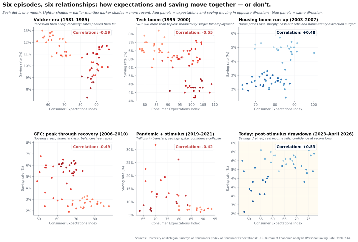
Six episodes. Six different patterns. Read panel by panel.

The Volcker era (1981-1985). Coming out of two recessions, Paul Volcker's Fed had broken inflation and rates were starting to fall. Consumer expectations surged from their 1980 lows. The saving rate, which had risen sharply during the recessions, dropped as households resumed normal spending. Expectations up, saving down — the textbook pattern of a recovery from a major shock. The correlation: −0.59.

The tech boom (1995-2000). The S&P 500 more than tripled. Productivity growth accelerated. The labor market reached full employment. Households watched their 401(k) balances climb and spent against them — a textbook wealth-effect story, just as Modigliani would predict. Expectations climbed; the saving rate fell from above 7% to roughly 4%. The correlation: −0.55.

The housing boom run-up (2003-2007). This is the only positive-correlation episode in the top row of the chart. Home prices rose sharply, and households extracted equity through cash-out refinancing and home-equity lines. Unlike the tech boom, the relationship turns positive in this window: months with higher expectations tended to coincide with somewhat higher saving rates, even though the saving rate remained historically low and both series weakened by the end of 2007. The correlation: +0.48.

The global financial crisis (2006-2010). Home prices collapsed. Wealth evaporated. Expectations cratered. Simultaneously, households slashed spending and rebuilt savings — buffer-stock behavior on a massive scale. Expectations fell as saving rose. The correlation: −0.49.

Pandemic plus stimulus (2019-2021). Trillions of dollars in transfer payments hit household balance sheets. The saving rate spiked above 30% in April 2020. Meanwhile, expectations collapsed under uncertainty about the virus, the economy, and household income. Expectations and saving moved in dramatic opposite directions, driven by an external transfer rather than household choices. The correlation: −0.42.

Today (2023-April 2026). The post-stimulus drawdown. The accumulated savings buffer has been spent down. Real disposable income has fallen for three consecutive months. The saving rate has dropped from above 5% in early 2025 to 2.6% in April 2026. Consumer expectations have fallen alongside it — to the lowest reading ever recorded in May. The correlation: +0.53. (Saving-rate data run through April 2026; Michigan expectations are available through May.)

What this chart is actually saying

The relationship between expectations and saving is not stable. It depends on which force is dominating household behavior.

When wealth gains are dominant — equity markets in the late 1990s — households can spend out of higher net worth while feeling more confident. Expectations rise, saving falls. Opposite directions.

When stimulus or transfers dominate — the pandemic — households can save the windfall while still feeling pessimistic about the underlying economy. Expectations collapse, saving rises. Opposite directions.

When a financial crisis hits — 2008 — households were forced to cut spending and rebuild savings defensively as incomes fell and expectations cratered. Expectations fall, saving rises. Opposite directions.

Today looks different.

The current correlation of +0.53 means expectations and saving are moving together. But the direction matters: both are falling.

That same +0.53 signature looks like the 2003-2007 housing run-up at first glance. The numbers are close, the visual pattern in the panels is close — but the mechanics are nearly opposite.

In 2003-2007, expectations and saving drifted together because perceived paper wealth — housing equity — was expanding. Households could comfortably lower their active saving rate because their unrealized wealth was growing in the background. Same signature, expansionary balance sheet.

Today, expectations and saving are moving together under duress. Real disposable income is falling, savings buffers have been spent down, and households are running down what cushion remains while becoming more pessimistic. Same signature, contracting balance sheet.

The same statistical relationship between expectations and saving can sit on opposite sides of the same coin.

If households were saving less because they expected stronger future income, we should see expectations improving. We do not. Expectations are at record lows, and more households expect income to weaken than improve.

What fits best is the buffer-stock story.

When households have a cushion, they can absorb shocks without immediately cutting spending. But when current income weakens and the cushion is thin, they smooth consumption by drawing down liquid savings before fully cutting back. Habit persistence reinforces this — cutting a standard of living downward is harder, behaviorally, than the formal math of buffer-stock smoothing alone would predict. That is what the data show now: real disposable income is falling, the saving rate is falling, and expectations are falling with it.

The chart does not prove the mechanism. But it does rule out the simplest optimism story. A falling saving rate alongside collapsing expectations looks more like pressure-driven dissaving.

That is the broader lesson: a falling saving rate does not have one meaning. It can reflect optimism, wealth effects, government transfers, balance-sheet repair, or pressure-driven dissaving.

What to watch next

Both possible futures from here are uncomfortable, and they live in different parts of the income distribution.

At the top, the wealth-effect-driven consumption strength could unwind if equities correct. Top-quintile households have been carrying a disproportionate share of aggregate consumption. Dallas Fed estimates suggest the top 20% of earners accounted for roughly 57% of overall consumption from 2020 through mid-2025, while the New York Fed's Economic Heterogeneity Indicators show consumer spending diverging sharply across household groups since 2023. These households are also the most exposed to changes in asset prices. Spending strength built on wealth gains is fragile if those gains reverse.

At the bottom and middle, buffer-stock dissaving has a different limit: liquid savings can run out. The aggregate saving rate at 2.6% is very low by historical standards — the lowest since mid-2022 and back near the thin-cushion levels seen in parts of the mid-2000s. The aggregate masks the distributional reality: highest-income quintile households still have more asset-price support and balance-sheet room, while middle- and lower-income households appear much closer to their liquid-buffer limits. Households cannot maintain consumption out of depleted buffers indefinitely.

How long can households keep spending when real income is weakening and savings buffers are thinner? That is the question for the rest of 2026.

Subscribe to get the next post.

Sources: University of Michigan, Surveys of Consumers (Index of Consumer Sentiment, Index of Consumer Expectations); U.S. Bureau of Economic Analysis, Personal Income and Outlays, April 2026; Personal Income and Its Disposition, Table 2.6 (full historical series); Federal Reserve Bank of New York, Economic Heterogeneity Indicators.